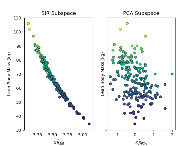
Comparing PCA with Sliced Inverse Regression¶

import matplotlib.pyplot as plt

from sklearn.decomposition import PCA

from sliced.datasets import load_athletes
from sliced import SlicedInverseRegression

X, y = load_athletes()

# fit SIR model
sir = SlicedInverseRegression(n_slices=11).fit(X, y)
X_sir = sir.transform(X)

# fit PCA
pca = PCA(random_state=123).fit(X, y)
X_pca = pca.transform(X)

f, (ax1, ax2) = plt.subplots(1, 2, sharey=True)

ax1.scatter(X_sir[:, 0], y, c=y, cmap='viridis', linewidth=0.5, edgecolor='k')
ax1.set_title('SIR Subspace')
ax1.set_xlabel("$X\hat{\\beta}_{SIR}$")
ax1.set_ylabel("Lean Body Mass (kg)")

ax2.scatter(X_pca[:, 0], y, c=y, cmap='viridis', linewidth=0.5, edgecolor='k')
ax2.set_title('PCA Subspace')
ax2.set_xlabel("$X\hat{\\beta}_{PCA}$")
ax2.set_ylabel("Lean Body Mass (kg)")

plt.show()