Quick Start¶

Joshua Loyal, January 2018

In [1]:

%matplotlib inline

import numpy as np
import matplotlib.pyplot as plt
import matplotlib as mpl

from mpl_toolkits.mplot3d import Axes3D

mpl.rcParams['figure.figsize'] = (10, 8)

The sliced package helps you find low dimensional information in your high dimensional data. Furthermore, this information is relevant to the problem’s target variable.

For example, consider the following data generating process:

$\beta = (1, 1, 0, 0, 0, 0, 0, 0, 0, 0)^T$

$X \overset{iid}\sim N(0, 1), \quad \epsilon \overset{iid}\sim N(0, 0.5)$

$Y = 0.125 \cdot (X\beta)^3 + \epsilon$

Where $X$ is a 10-dimensional feature matrix. Notice that $Y$ only depends on $X$ through a linear combination of the first two features: $X_1 + X_2$ . This is a one-dimensional subspace. The methods in sliced try to find this subspace.

Let’s see how sliced finds this subspace. We start by generating the dataset described above. It is example dataset included in the sliced package:

In [2]:

from sliced.datasets import make_cubic

X, y = make_cubic(random_state=123)
X.shape

Out[2]:

(500, 10)

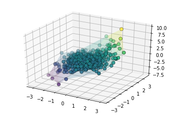
The surface in three-dimensions is displayed below. Note that we normally do not know that $X_1$ and $X_2$ contain all the information about the target.

In [3]:

ax = plt.axes(projection='3d')
ax.plot_trisurf(X[:, 0], X[:, 1], y,
                cmap='viridis', alpha=0.2, edgecolor='none')
ax.scatter3D(X[:, 0], X[:, 1], y, c=y,
             cmap='viridis', edgecolor='k', s=50, linewidth=0.5)

Out[3]:

<mpl_toolkits.mplot3d.art3d.Path3DCollection at 0x2b1f62032908>

To learn a low dimensional representation we use the SlicedInverseRegression algorithm found in sliced. Fitting the algorithms is easy since it adheres to the sklearn transformer API. A single hyperparameter n_directions indicates the dimension of the subspace. In this case we want a single direction, so we set n_directions=1. The directions_ attribute stores the estimated direction of the subspace once the algorithm is fit. The following fits the SIR algorithm:

In [4]:

from sliced import SlicedInverseRegression

sir = SlicedInverseRegression(n_directions=1)
sir.fit(X, y)

Out[4]:

SlicedInverseRegression(alpha=None, copy=True, n_directions=1, n_slices=10)

To actually perform the dimension reduction we call the transform method on the data:

In [5]:

X_sir = sir.transform(X)

plt.scatter(X_sir[:, 0], y,
            c=y, cmap='viridis', edgecolors='k', s=80)
plt.xlabel('$X\\beta_{sir}$')
plt.ylabel('y')

Out[5]:

Text(0,0.5,'y')

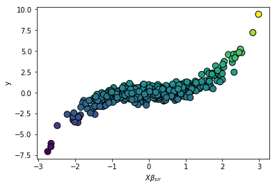
../_images/notebooks_quickstart_10_1.png

The cubic structure is accuratly identified with a single feature. sliced reduced the dimension of the dataset from 10 to 1!